Getting started
To get you up and running, the following guides highlights the basics of the API for ensemble classes, model selection and visualization.
| Guides | Content |
|---|---|
| Ensemble guide | how to build, fit and predict with an ensemble |
| Model selection guide | how to compare several estimators in one go |
| Visualization guide | plotting functionality |
For more more in-depth material and advanced usage, see Tutorials.
Preliminaries
We use the following setup throughout:
import numpy as np
from pandas import DataFrame
from sklearn.metrics import f1_score
from sklearn.datasets import load_iris

seed = 2017
np.random.seed(seed)

def f1(y, p): return f1_score(y, p, average='micro')

data = load_iris()
idx = np.random.permutation(150)
X = data.data[idx]
y = data.target[idx]
Ensemble guide
Building an ensemble
Instantiating a fully specified ensemble is straightforward and requires three steps: first create the instance, second add the intermediate layers, and finally the meta estimator.
from mlens.ensemble import SuperLearner
from sklearn.linear_model import LogisticRegression
from sklearn.ensemble import RandomForestClassifier
from sklearn.svm import SVC

# --- Build ---

# Passing a scoring function will create cv scores during fitting
# the scorer should be a simple function accepting to vectors and returning a scalar
ensemble = SuperLearner(scorer=f1, random_state=seed)

# Build the first layer
ensemble.add([RandomForestClassifier(random_state=seed), SVC()])

# Attach the final meta estimator
ensemble.add_meta(LogisticRegression())

# --- Use ---

# Fit ensemble
ensemble.fit(X[:75], y[:75])

# Predict
preds = ensemble.predict(X[75:])
To check the performance of estimator in the layers, call the scores_
attribute. The attribute can be wrapped in a pandas.DataFrame
for a tabular format.
>>> DataFrame(ensemble.scores_)
                                score_mean  score_std
layer-1 randomforestclassifier    0.839260   0.055477
        svc                       0.894026   0.051920
To round off, let’s see how the ensemble as a whole fared.
>>> f1(preds, y[75:])
0.95999999999999996
Multi-layer ensembles
With each call to the add method, another layer is added to the ensemble.
Note that all ensembles are sequential in the order layers are added. For
instance, in the above example, we could add a second layer as follows.
ensemble = SuperLearner(scorer=f1, random_state=seed, verbose=True)

# Build the first layer
ensemble.add([RandomForestClassifier(random_state=seed), LogisticRegression()])

# Build the second layer
ensemble.add([LogisticRegression(), SVC()])

# Attach the final meta estimator
ensemble.add_meta(SVC())
We now fit this ensemble in the same manner as before:
>>> ensemble.fit(X[:75], y[:75])
Processing layers (3)

Fitting layer-1
[Parallel(n_jobs=-1)]: Done   7 out of   6 | elapsed:    0.1s remaining:   -0.0s
[Parallel(n_jobs=-1)]: Done   7 out of   6 | elapsed:    0.1s remaining:   -0.0s
[Parallel(n_jobs=-1)]: Done   7 out of   6 | elapsed:    0.1s remaining:   -0.0s
[Parallel(n_jobs=-1)]: Done   7 out of   6 | elapsed:    0.1s remaining:   -0.0s
[Parallel(n_jobs=-1)]: Done   7 out of   6 | elapsed:    0.1s remaining:   -0.0s
[Parallel(n_jobs=-1)]: Done   6 out of   6 | elapsed:    0.1s finished
layer-1 Done | 00:00:00

Fitting layer-2
[Parallel(n_jobs=-1)]: Done   7 out of   6 | elapsed:    0.0s remaining:   -0.0s
[Parallel(n_jobs=-1)]: Done   7 out of   6 | elapsed:    0.1s remaining:   -0.0s
[Parallel(n_jobs=-1)]: Done   7 out of   6 | elapsed:    0.1s remaining:   -0.0s
[Parallel(n_jobs=-1)]: Done   7 out of   6 | elapsed:    0.1s remaining:   -0.0s
[Parallel(n_jobs=-1)]: Done   7 out of   6 | elapsed:    0.1s remaining:   -0.0s
[Parallel(n_jobs=-1)]: Done   6 out of   6 | elapsed:    0.1s finished
layer-2 Done | 00:00:00

Fitting layer-3
[Parallel(n_jobs=-1)]: Done   1 out of   1 | elapsed:    0.0s finished
[Parallel(n_jobs=-1)]: Done   1 out of   1 | elapsed:    0.0s finished
layer-3 Done | 00:00:00

Fit complete | 00:00:00
Similarly with predictions:
>>> preds = ensemble.predict(X[75:])
Processing layers (3)

Predicting layer-1
[Parallel(n_jobs=-1)]: Done   2 out of   2 | elapsed:    0.0s finished
layer-1 Done | 00:00:00

Predicting layer-2
[Parallel(n_jobs=-1)]: Done   2 out of   2 | elapsed:    0.0s finished
layer-2 Done | 00:00:00

Predicting layer-3
[Parallel(n_jobs=-1)]: Done   1 out of   1 | elapsed:    0.0s finished
layer-3 Done | 00:00:00

Done | 00:00:00
The design of the scores_ attribute allows an intuitive overview of how
the base learner’s perform in each layer.
>>> DataFrame(ensemble.scores_)
                                score_mean  score_std
layer-1 logisticregression        0.735420   0.156472
        randomforestclassifier    0.839260   0.055477
layer-2 logisticregression        0.668208   0.115576
        svc                       0.893314   0.001422
Model selection guide
The work horse class is the Evaluator, which allows you to
grid search several models in one go across several preprocessing pipelines.
The evaluator class pre-fits transformers, thus avoiding fitting the same
preprocessing pipelines on the same data repeatedly.
The following example evaluates a Naive Bayes estimator and a K-Nearest-Neighbor estimator under three different preprocessing scenarios: no preprocessing, standard scaling, and subset selection. In the latter case, preprocessing is constituted by selecting a subset of features.
The scoring function
An important note is that the scoring function must be wrapped by
make_scorer(), to ensure all scoring functions behave similarly regardless
of whether they measure accuracy or errors. To wrap a function, simple do:
from mlens.metrics import make_scorer
f1_scorer = make_scorer(f1_score, average='micro', greater_is_better=True)
The make_scorer wrapper
is a copy of the Scikit-learn’s sklearn.metrics.make_scorer(), and you
can import the Scikit-learn version as well.
Note however that to pickle the Evaluator, you must import
make_scorer from mlens.
A simple evaluation
Before throwing preprocessing into the mix, let’s see how to evaluate a set of
estimator. First, we need a list of estimator and a dictionary of parameter
distributions that maps to each estimator. The estimators should be put in a
list, either as is or as a named tuple ((name, est)). If you don’t name
the estimator, the Evaluator will automatically name the model as the
class name in lower case. This name must be the key in the parameter
dictionary. Let’s see how to set this up:
from mlens.model_selection import Evaluator
from sklearn.naive_bayes import GaussianNB
from sklearn.neighbors import KNeighborsClassifier

from scipy.stats import randint

# Here we name the estimators ourselves
ests = [('gnb', GaussianNB()), ('knn', KNeighborsClassifier())]

# Now we map parameters to these
# The gnb doesn't have any parameters so we can skip it
pars = {'n_neighbors': randint(2, 20)}
params = {'knn': pars}
We can now run an evaluation over these estimators and parameter distributions
by calling the evaluate method.
>>> evaluator = Evaluator(f1_scorer, cv=10, random_state=seed, verbose=1)
>>> evaluator.evaluate(X, y, ests, params, n_iter=10)
Evaluating 2 models for 10 parameter draws over 10 CV folds, totalling 200 fits
[Parallel(n_jobs=-1)]: Done 110 out of 110 | elapsed:    0.2s finished
Evaluation done | 00:00:00
The full history of the evaluation can be found in cv_results. To compare
models with their best parameters, we can pass the summary attribute to
a pandas.DataFrame.
>>> DataFrame(evaluator.summary)
        test_score_mean  test_score_std  train_score_mean  train_score_std  fit_time_mean  fit_time_std               params
gnb         0.960000        0.032660          0.957037         0.005543          0.001298      0.001131                   {}
knn         0.966667        0.033333          0.980000         0.004743          0.000866      0.001001  {'n_neighbors': 15}
Preprocessing
Next, suppose we want to compare the models across a set of preprocessing pipelines. To do this, we first need to specify a dictionary of preprocessing pipelines to run through. Each entry in the dictionary should be a list of transformers to apply sequentially.
from mlens.preprocessing import Subset
from sklearn.preprocessing import StandardScaler

# Map preprocessing cases through a dictionary
preprocess_cases = {'none': [],
                    'sc': [StandardScaler()],
                    'sub': [Subset([0, 1])]
                    }
We can either fit the preprocessing pipelines and estimators in one go using the
fit method, or we can pre-fit the transformers before we decide on
estimators.
This can be helpful if the preprocessing is time-consuming, for instance if
the preprocessing pipeline is an EnsembleTransformer. This class
mimics how an ensemble creates prediction matrices during fit and predict
calls, and can thus be used as a preprocessing pipeline to evaluate different
candidate meta learners. See the Ensemble model selection tutorial for
an example. To explicitly fit preprocessing pipelines, call preprocess.
>>> evaluator.preprocess(X, y, preprocess_cases)
Preprocessing 3 preprocessing pipelines over 10 CV folds
[Parallel(n_jobs=-1)]: Done  30 out of  30 | elapsed:    0.2s finished
Preprocessing done | 00:00:00
Model Selection across preprocessing pipelines
To evaluate the same set of estimators across all pipelines with the same parameter distributions, there is no need to take any heed of the preprocessing pipeline, just carry on as in the simple case:
>>> evaluator.evaluate(X, y, ests, params, n_iter=10)
>>> DataFrame(evaluator.summary)
          test_score_mean  test_score_std  train_score_mean  train_score_std  fit_time_mean  fit_time_std               params
none gnb         0.960000        0.032660          0.957037         0.005543       0.003507      0.003547                   {}
     knn         0.960000        0.044222          0.974815         0.007554       0.002421      0.003270  {'n_neighbors': 11}
sc   gnb         0.960000        0.032660          0.957037         0.005543       0.000946      0.000161                   {}
     knn         0.960000        0.044222          0.965185         0.003395       0.000890      0.000568   {'n_neighbors': 8}
sub  gnb         0.780000        0.133500          0.791111         0.019821       0.000658      0.000109                   {}
     knn         0.786667        0.122202          0.825926         0.016646       0.000385      0.000063  {'n_neighbors': 11}
You can also map different estimators to different preprocessing folds, and map different parameter distribution to each case.
# We will map two different parameter distributions
pars_1 = {'n_neighbors': randint(20, 30)}
pars_2 = {'n_neighbors': randint(2, 10)}
params = {('sc', 'knn'): pars_1,
          ('none', 'knn'): pars_2,
          ('sub', 'knn'): pars_2}

# We can map different estimators to different cases
ests_1 = [('gnb', GaussianNB()), ('knn', KNeighborsClassifier())]
ests_2 = [('knn', KNeighborsClassifier())]
estimators = {'sc': ests_1,
              'none': ests_2,
              'sub': ests_1}
To run cross-validation, call the evaluate method.
Make sure to specify the number of parameter draws to evaluate
(the n_iter parameter).
>>> evaluator.evaluate(X, y, estimators, params, n_iter=10)
Evaluating 6 estimators for 10 parameter draws 10 CV folds, totalling 600 fits
[Parallel(n_jobs=-1)]: Done 600 out of 600 | elapsed:    1.0s finished
Evaluation done | 00:00:01
As before, we can summarize the evaluation in a nice DataFrame.
>>> DataFrame(evaluator.summary)
       test_score_mean  test_score_std  train_score_mean  train_score_std    fit_time_mean  fit_time_std               params
none knn         0.966667        0.044721          0.960741         0.007444         0.001718      0.003330   {'n_neighbors': 3}
sc   gnb         0.960000        0.032660          0.957037         0.005543         0.000926      0.000139                   {}
     knn         0.940000        0.055377          0.962963         0.005738         0.000430      0.000035  {'n_neighbors': 20}
sub  gnb         0.780000        0.133500          0.791111         0.019821         0.000869      0.000126                   {}
     knn         0.800000        0.126491          0.837037         0.014815         0.000426      0.000068   {'n_neighbors': 9}
The Evaluator provides a one-stop-shop for comparing many different
models in various configurations, and is a critical tool to leverage when
building complex ensembles. It is especially helpful in combination with the
EnsembleTransformer, which allows use to evaluate the next layer
of an ensemble or a set of potential meta learners without having to run the
entire ensemble every time. As such, it provides a way to perform greedy
layer-wise parameter tuning. For more details, see the Ensemble model selection tutorial.
Visualization guide
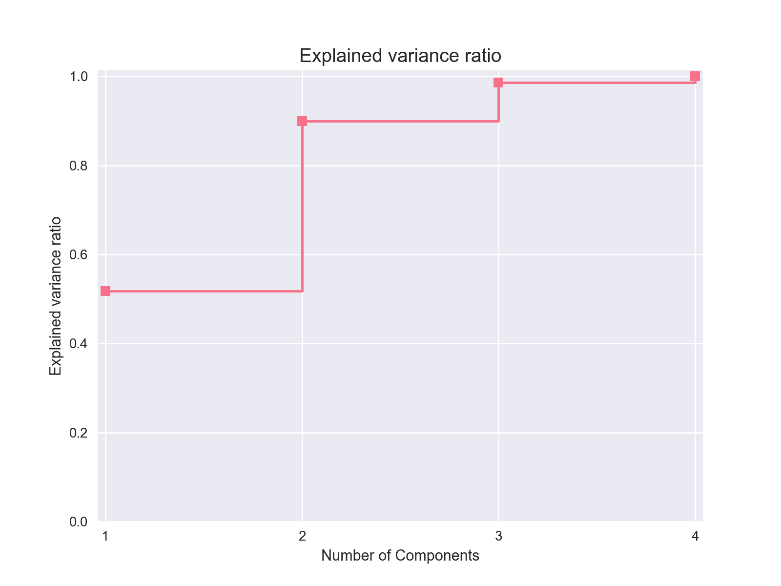
Explained variance plot
The exp_var_plot function
plots the explained variance from mapping a matrix X onto a smaller
dimension using a user-supplied transformer, such as the Scikit-learn
sklearn.decomposition.PCA transformer for
Principal Components Analysis.
>>> from mlens.visualization import exp_var_plot
>>> from sklearn.decomposition import PCA
>>>
>>> exp_var_plot(X, PCA(), marker='s', where='post')
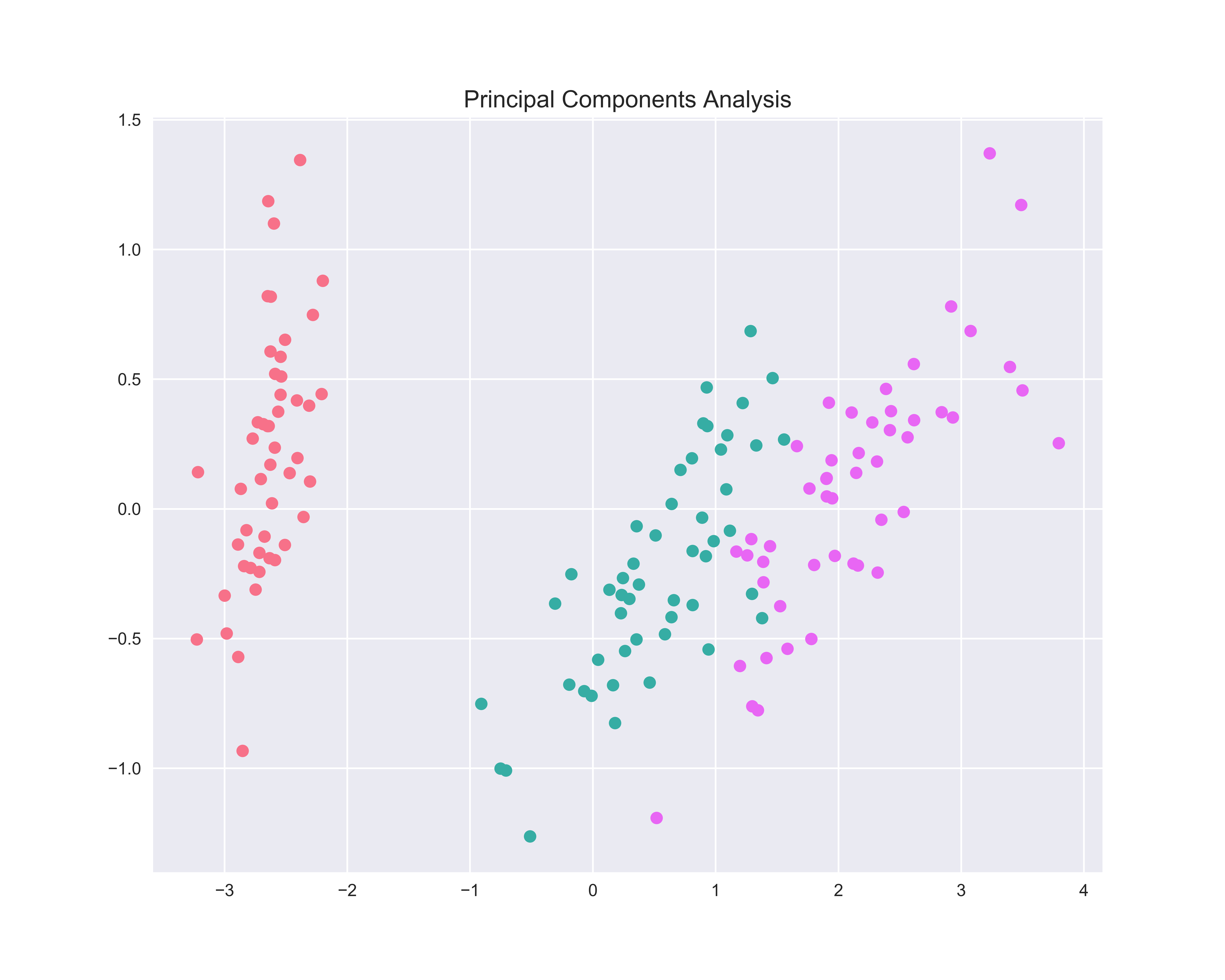
Principal Components Analysis plot
The pca_plot function
plots a PCA analysis or similar if n_components is one of [1, 2, 3].
By passing a class labels, the plot shows how well separated different classes
are.
>>> from mlens.visualization import pca_plot
>>> from sklearn.decomposition import PCA
>>>
>>> pca_plot(X, PCA(n_components=2), y=y)
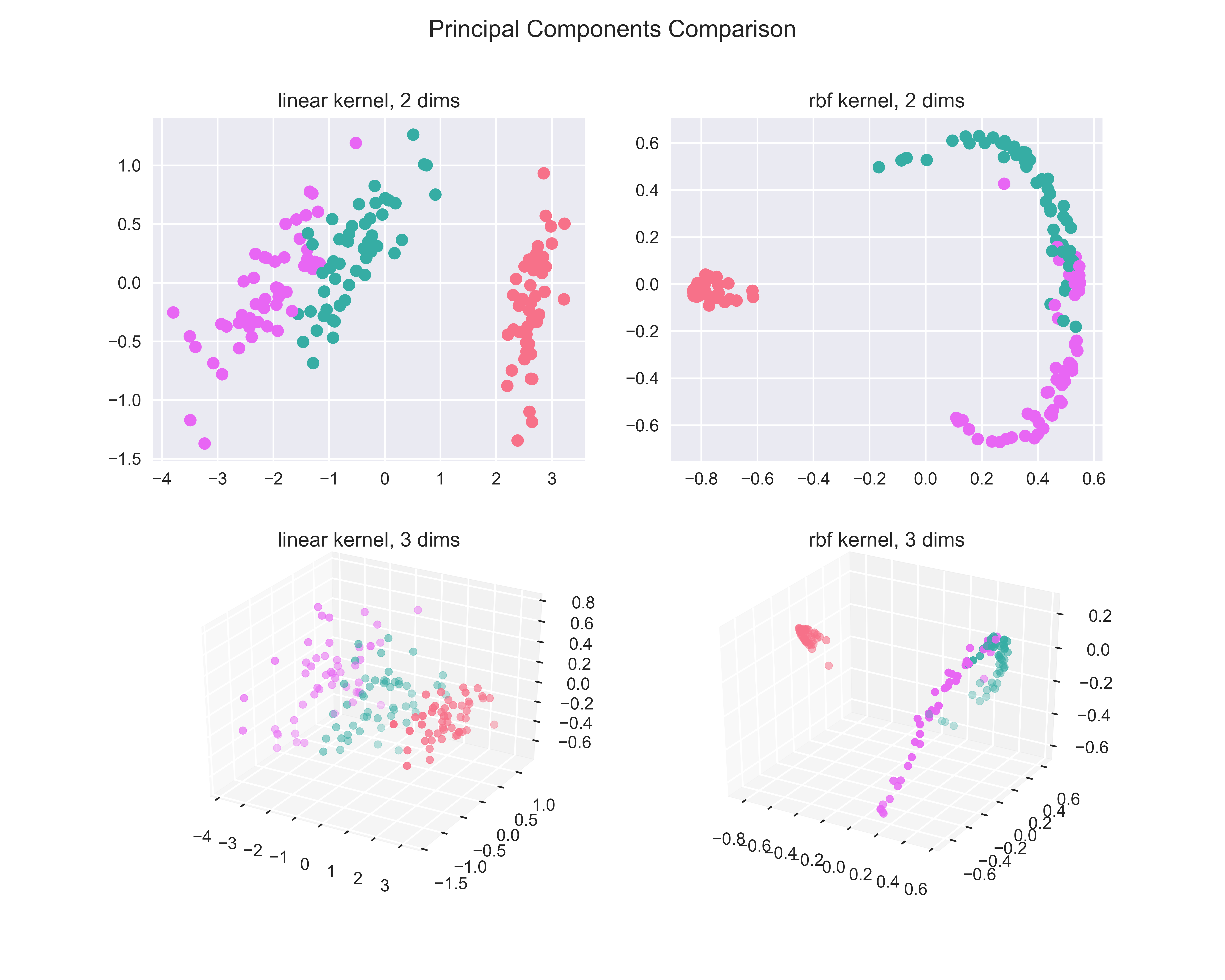
Principal Components Comparison plot
The pca_comp_plot function
plots a matrix of PCA analyses, one for each combination of
n_components=2, 3 and kernel='linear', 'rbf'.
>>> from mlens.visualization import pca_comp_plot
>>>
>>> pca_comp_plot (X, y)
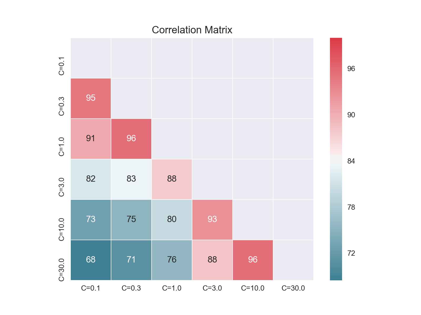
Correlation matrix plot
The corrmat function plots the lower triangle of
a correlation matrix and is adapted the Seaborn correlation matrix.
>>> from mlens.visualization import corrmat
>>>
>>> # Generate som different predictions to correlate
>>> params = [0.1, 0.3, 1.0, 3.0, 10, 30]
>>> preds = np.zeros((150, 6))
>>> for i, c in enumerate(params):
...    preds[:, i] = LogisticRegression(C=c).fit(X, y).predict(X)
>>>
>>> corr = DataFrame(preds, columns=['C=%.1f' % i for i in params]).corr()
>>> corrmat(corr)
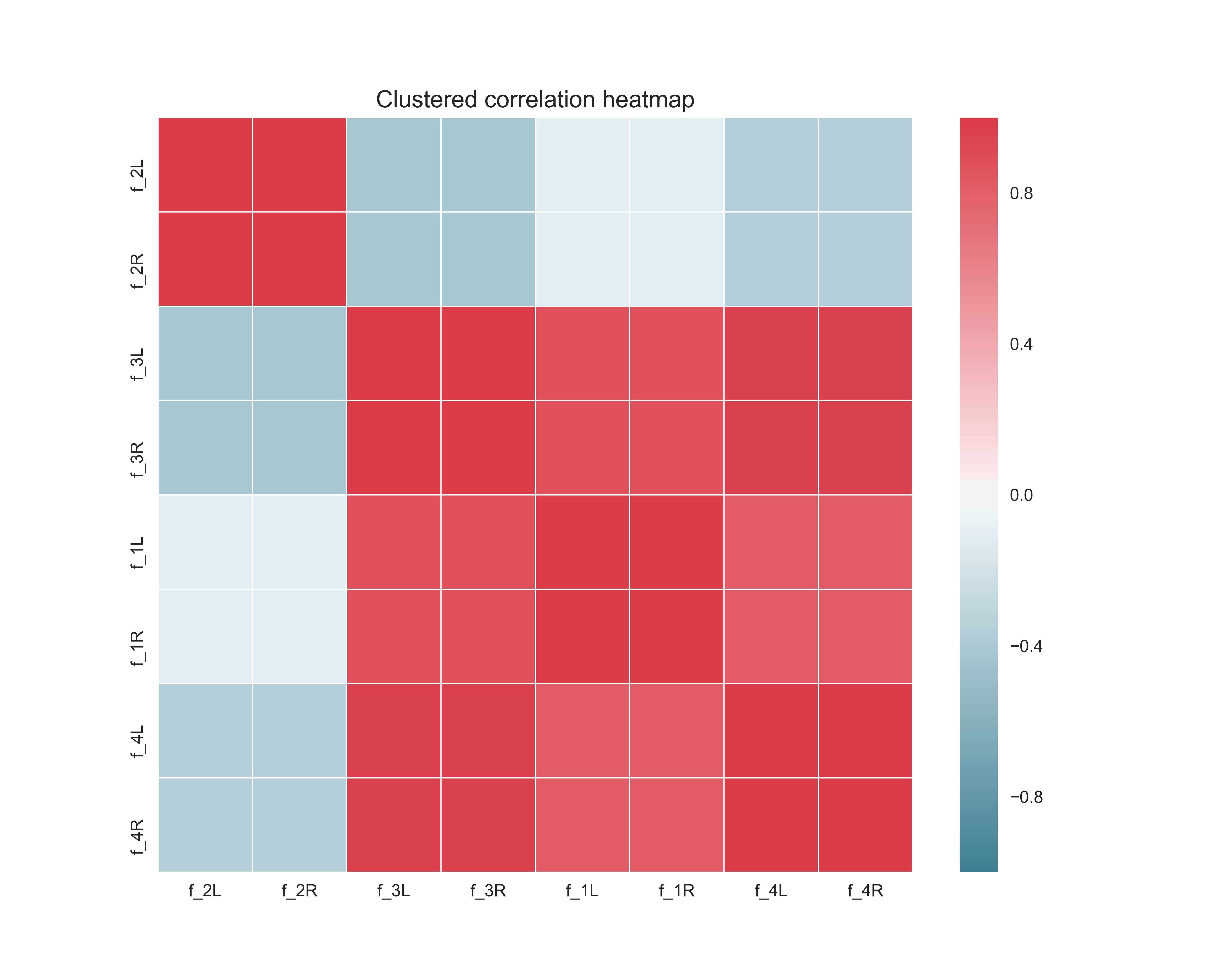
Clustered correlation heatmap plot
The clustered_corrmap function is similar to corrmat,
but differs in two respects. First, and most importantly, it uses a user
supplied clustering estimator to cluster the correlation matrix on similar
features, which can often help visualize whether there are blocks of highly
correlated features. Secondly, it plots the full matrix (as opposed to the
lower triangle).
>>> from mlens.visualization import clustered_corrmap
>>> from sklearn.cluster import KMeans
>>>
>>> Z = DataFrame(X, columns=['f_%i' %i for i in range(1, 5)])
>>>
>>> # We duplicate all features, note that the heatmap orders features
>>> # as duplicate pairs, and thus fully pick up on this duplication.
>>> corr = Z.join(Z, lsuffix='L', rsuffix='R').corr()
>>>
>>> clustered_corrmap(corr, KMeans())
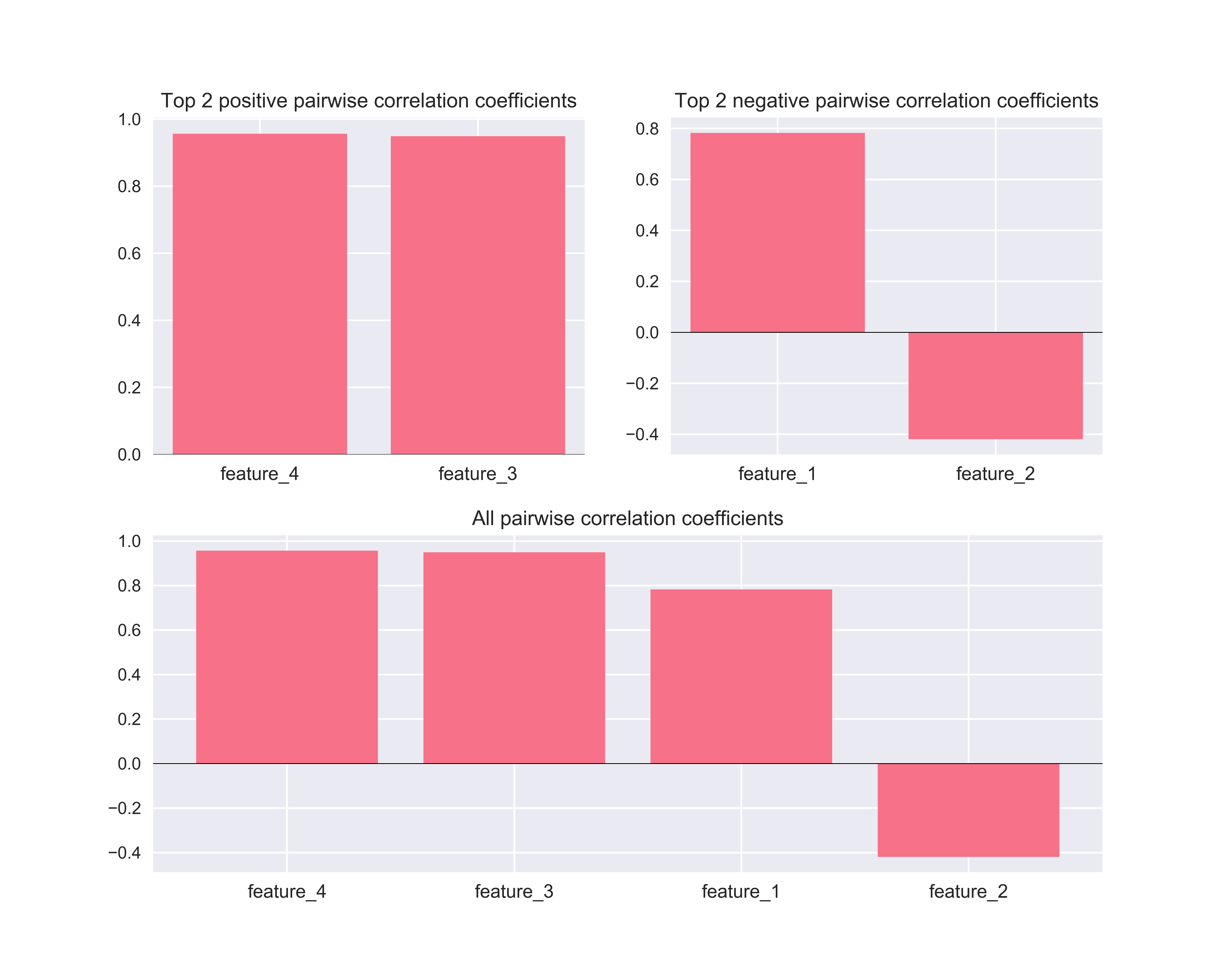
Input-Output correlations
The corr_X_y function gives a dashboard of
pairwise correlations between the input data (X) and the labels to be
predicted (y). If the number of features is large, it is advised to set
the no_ticks parameter to True, to avoid rendering an illegible
x-axis. Note that X must be a pandas.DataFrame.
>>> Z = DataFrame(X, columns=['feature_%i' %i for i in range(1, 5)])
>>> corr_X_y(Z, y, 2, no_ticks=False)